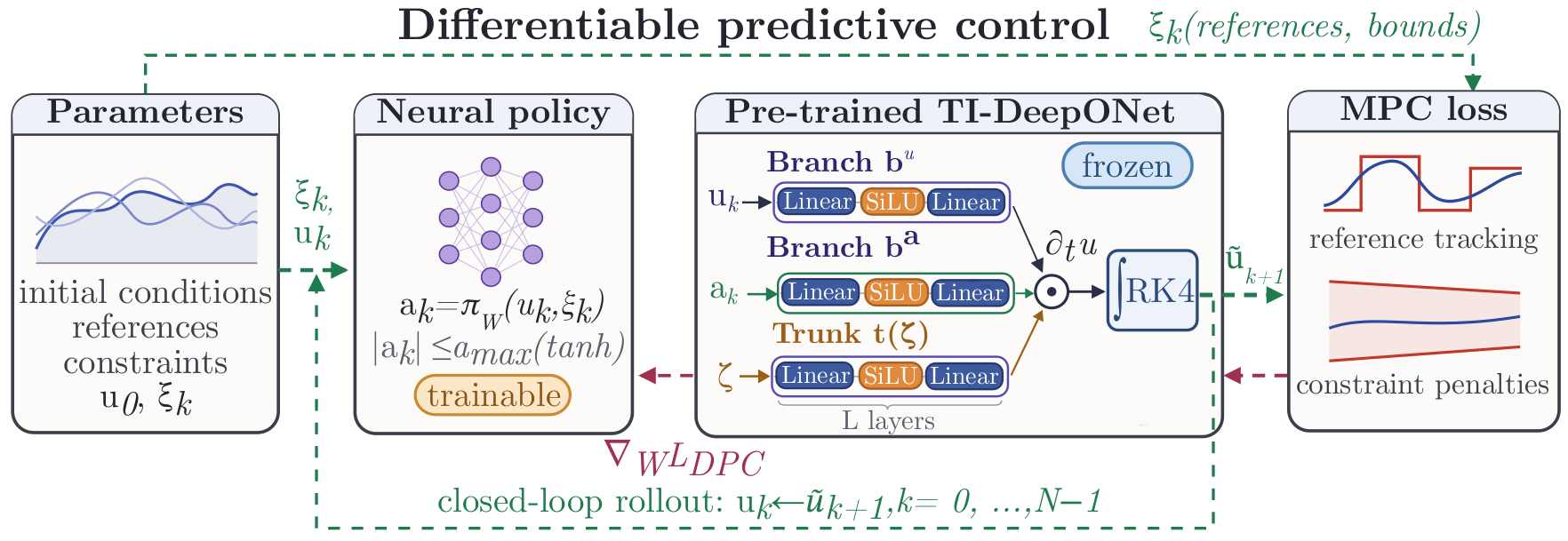
We present a data-driven control framework for partial differential equations (PDEs). Our approach integrates Time-Integrated Deep Operator Networks (TI-DeepONets) as differentiable PDE surrogate models within the Differentiable Predictive Control (DPC), a self-supervised learning framework for constrained neural control policies. The TI-DeepONet architecture learns temporal derivatives and couples them with numerical integrators, while the DPC algorithm uses automatic differentiation to compute policy gradients by backpropagating the expectations of the optimal control loss through the learned TI-DeepONet. This approach enables efficient offline optimization of neural policies without the need for online optimization or supervisory controllers. We empirically demonstrate the proposed method across diverse PDE systems, including the heat, the nonlinear Burgers', and the reaction-diffusion equations. The learned policies achieve target tracking, constraint satisfaction, and curvature minimization objectives, while generalizing across distributions of initial conditions and parameters. Moreover, we demonstrate four orders of magnitude acceleration at inference time compared to nonlinear model predictive control benchmarks. These results highlight the promise of operator learning for scalable model-based control of PDEs.
A TI-DeepONet predicts the temporal derivative of the state rather than the next state directly, and is composed with an RK4 integrator. Keeping the integrator explicit preserves temporal causality and limits error accumulation over long horizons. That is what makes the surrogate trustworthy enough to differentiate through for hundreds of steps.
The surrogate is frozen. The optimal-control loss is evaluated on a full closed-loop rollout and its gradient flows back through every integration step to the policy parameters. No labelled control data, no supervisory controller, and no optimization at deployment. The policy is a single forward pass.
Every system is actuated by Gaussian sources whose amplitudes the policy sets at each step: $f(x,t)=\sum_i c_i(t)\,\exp\!\left(-\frac{(x-x_i)^2}{2\sigma^2}\right)$
| System | Dynamics | Control objective | Policy |
|---|---|---|---|
| Heat | $\partial_t u = \nu\,\partial_{xx}u + f$ | Target tracking | $\pi(u_t,u^\ast)\to c\in\mathbb{R}^4$ |
| Burgers' | $\partial_t u + u\,\partial_x u = f$ | Shock mitigation minimize curvature $\lVert\partial_{xx}u\rVert^2$ |
$\pi(u_t)\to c\in\mathbb{R}^2$ |
| Reaction-diffusion | $\partial_t u = D\,\partial_{xx}u + r\,u(1-u) + f$ | Target tracking | $\pi(u_t,u^\ast)\to c\in\mathbb{R}^4$ |
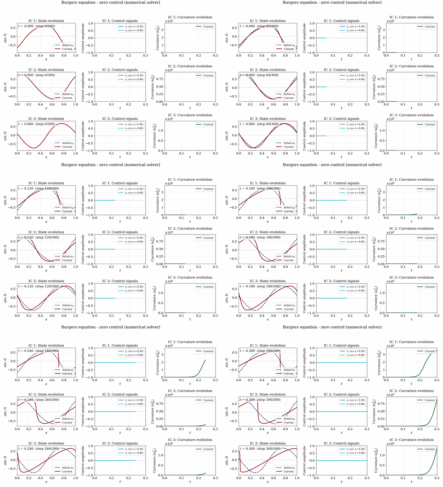
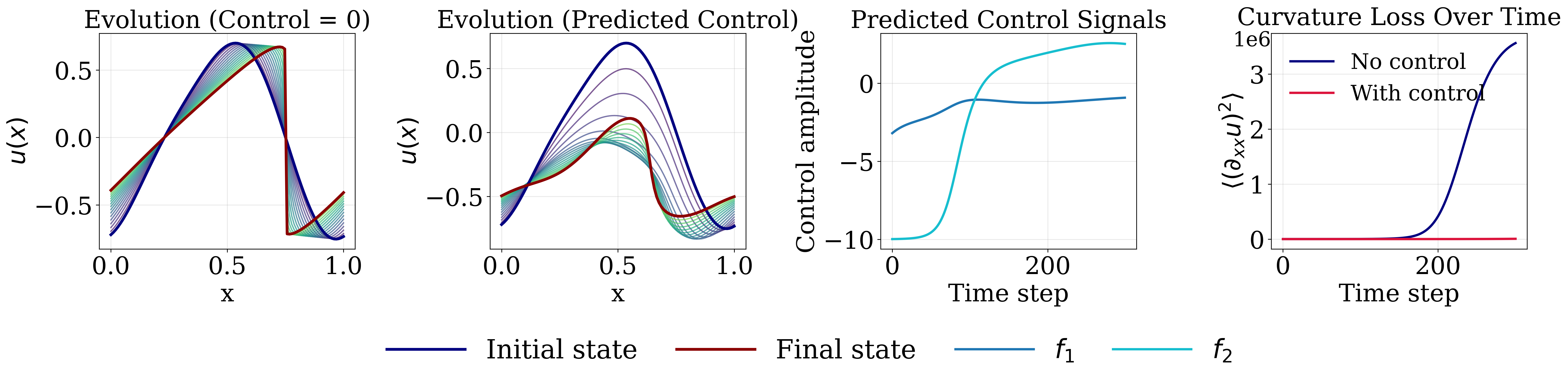
Burgers' is the outlier by design: there is no target state, so the policy observes only the current state and is rewarded purely for flattening curvature.
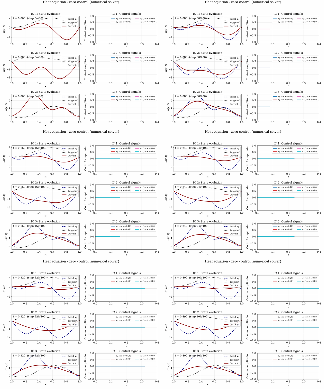
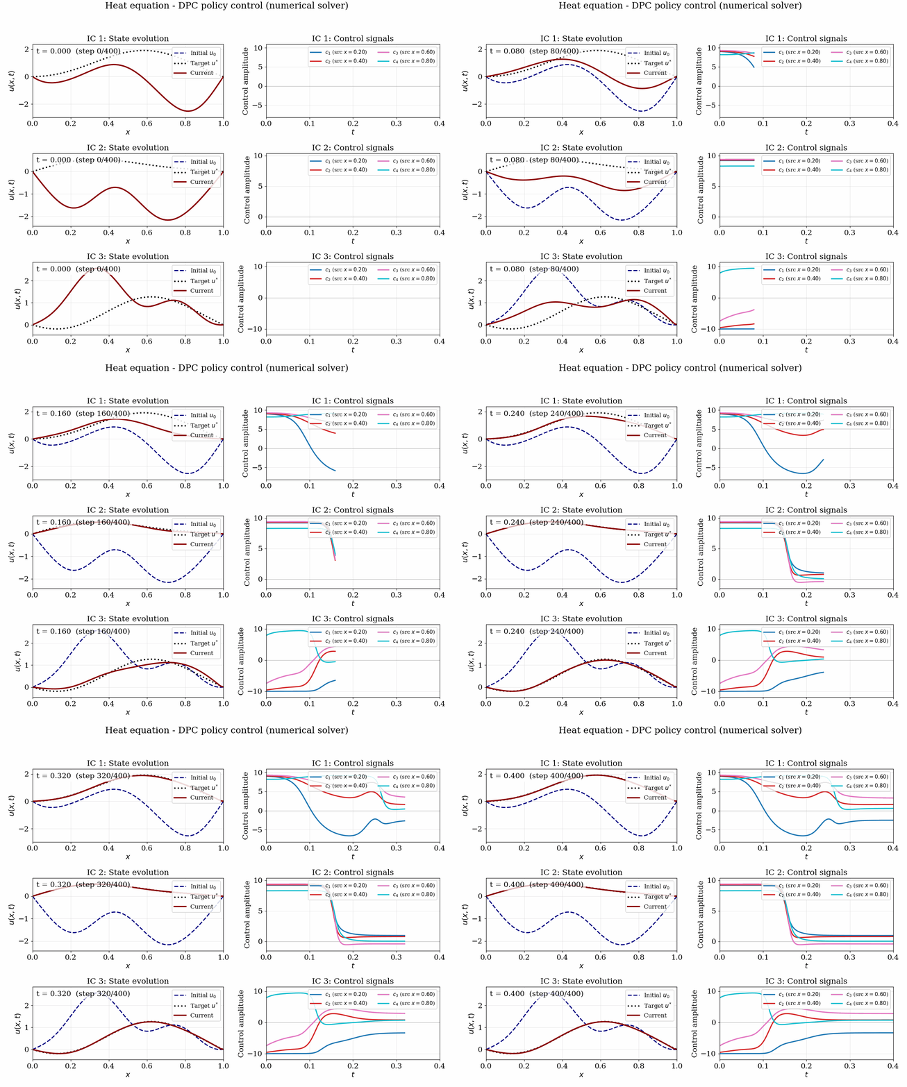
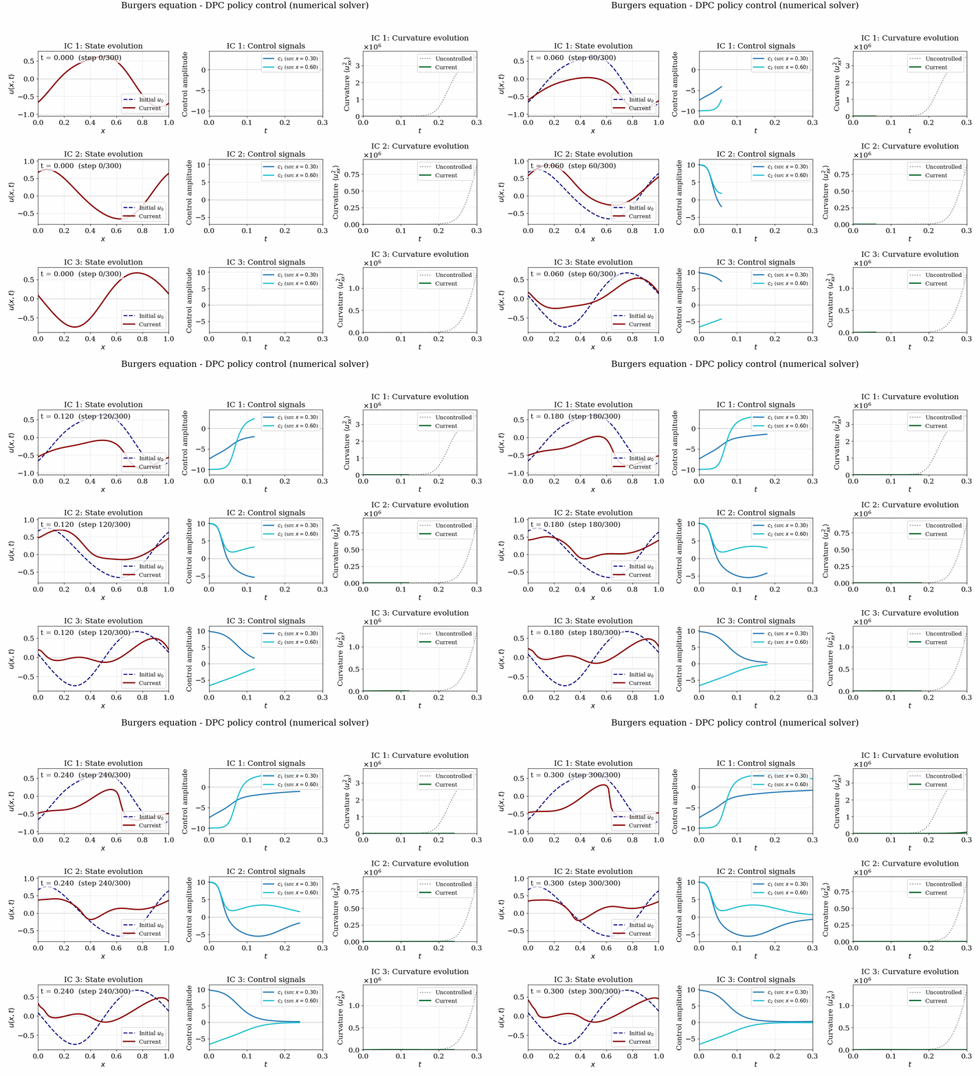
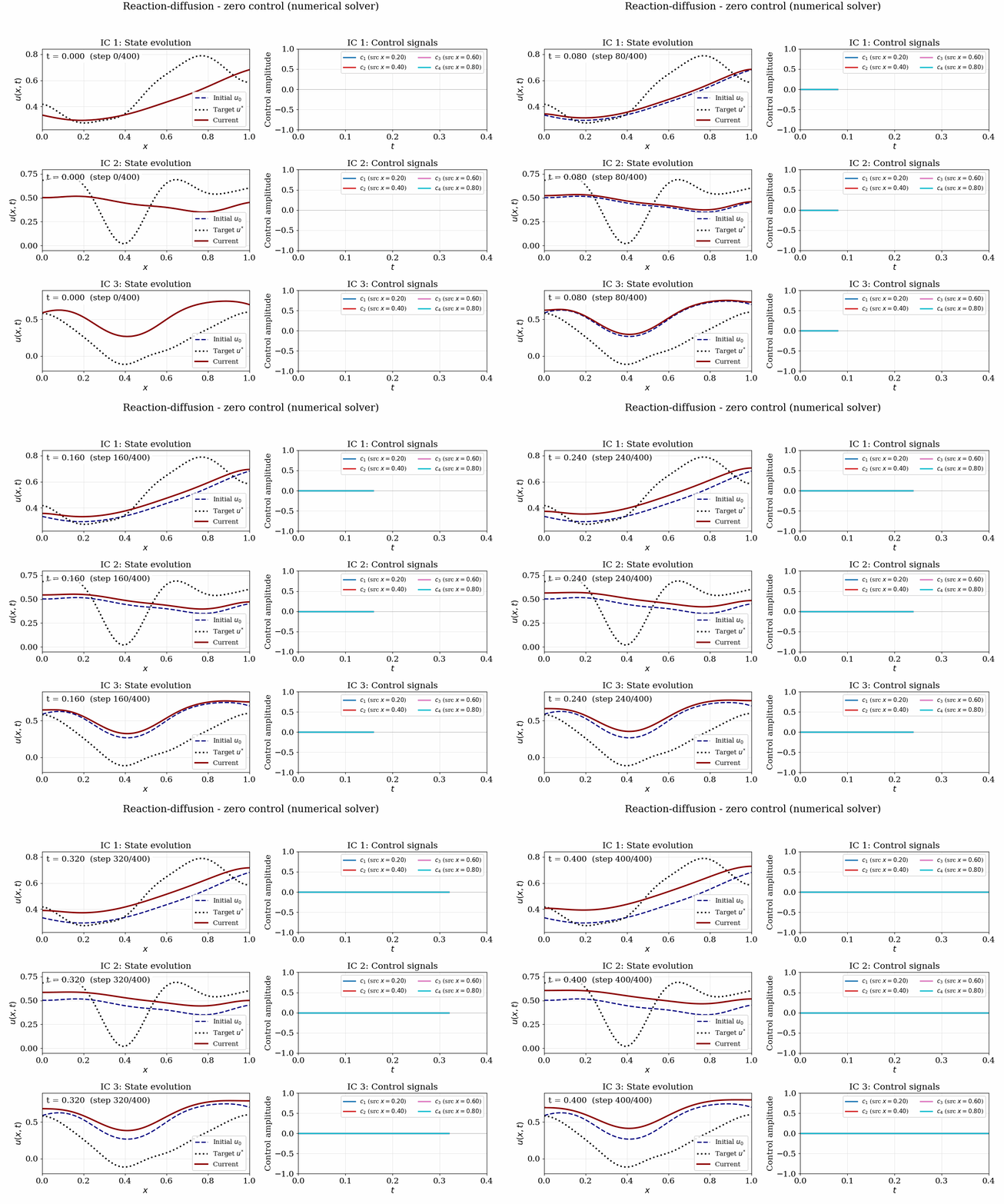
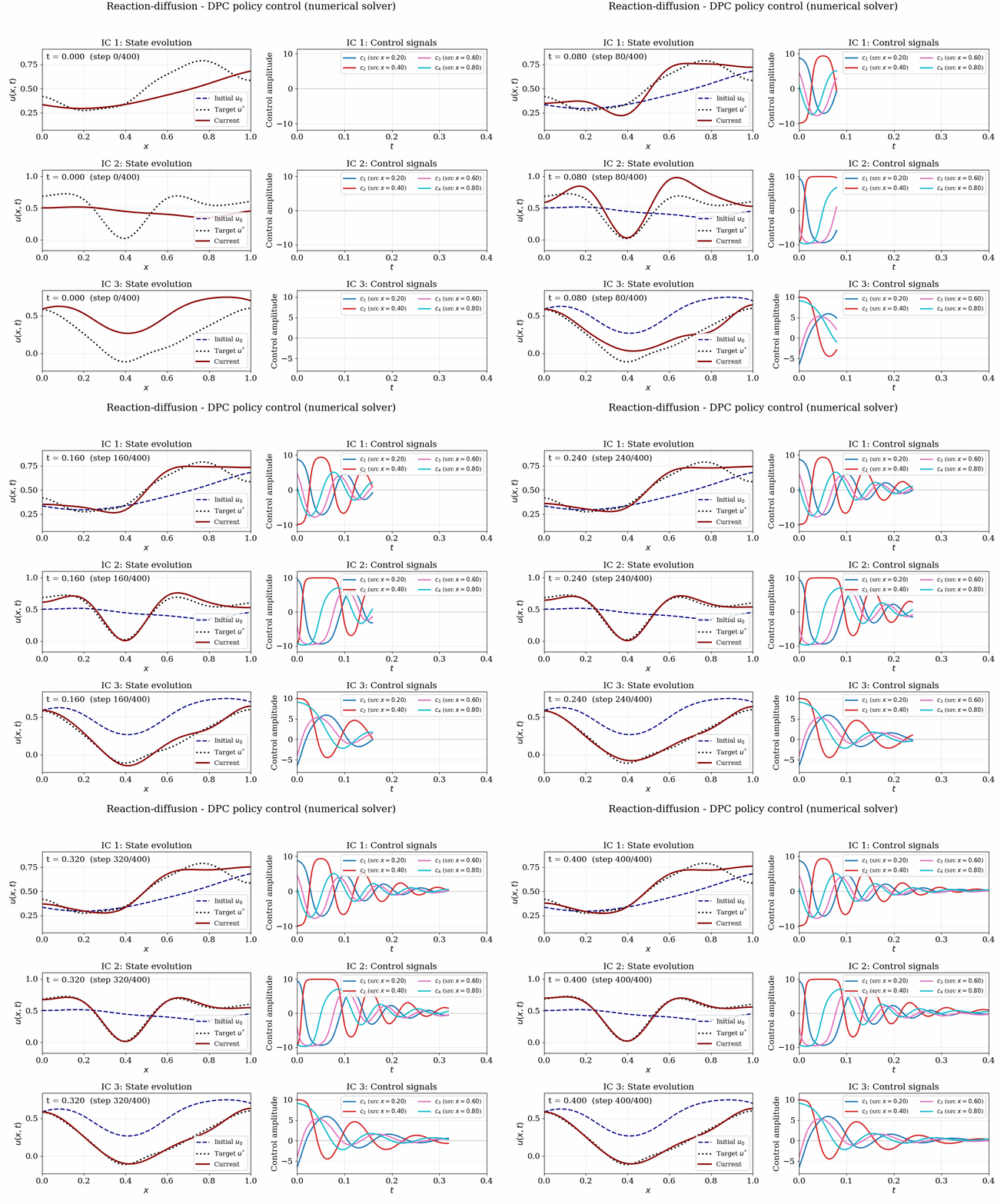
Each panel compares the uncontrolled evolution against the policy-controlled one, on initial conditions the policy has never seen. Use the arrows to switch between systems.
No control
Learned policy
No control
Learned policy
No control
Learned policy
Because the policy is a single forward pass, deployment costs a network evaluation instead of solving an optimization problem at every step. Against nonlinear MPC benchmarks the paper reports four orders of magnitude of acceleration.
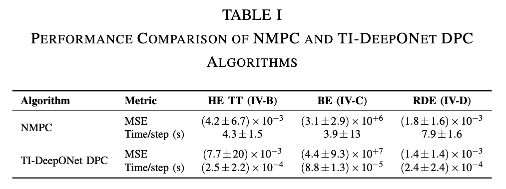
Nonlinear MPC needs seconds per control step because it solves an optimization problem online. The learned policy needs tenths of a millisecond, while reaching comparable tracking error. Across the three systems that is a speedup of roughly 1.7×10⁴, 4.4×10⁴ and 3.3×10⁴.
Policies are trained against the learned surrogate, then deployed on the true numerical solver. That is the real test of whether the surrogate was faithful enough to learn through.
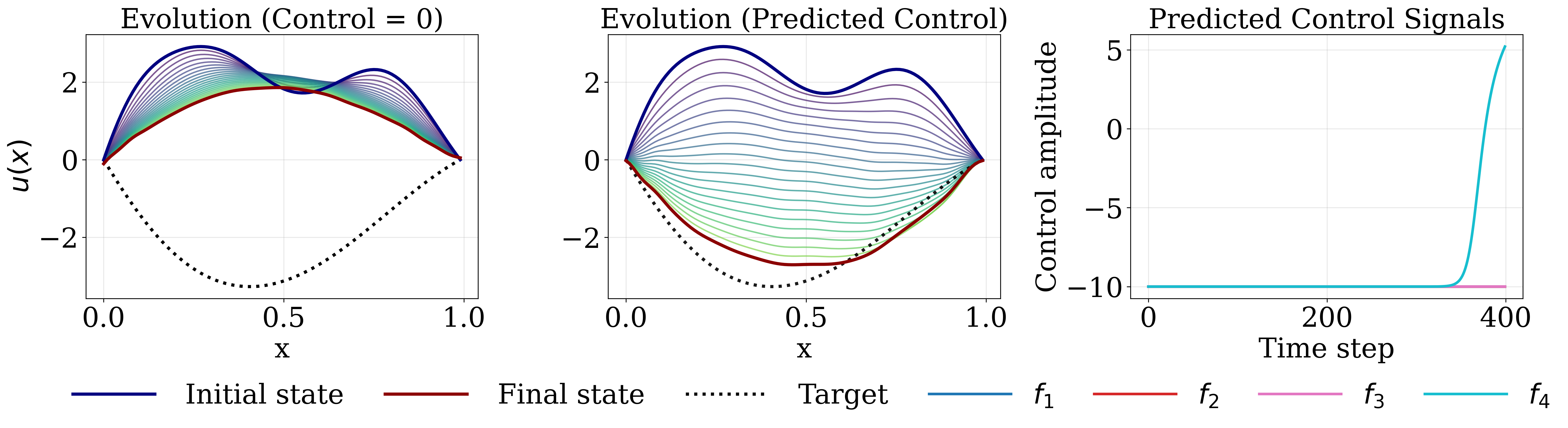
learned dynamics Policy-controlled vs. uncontrolled evolution with the applied control signals.
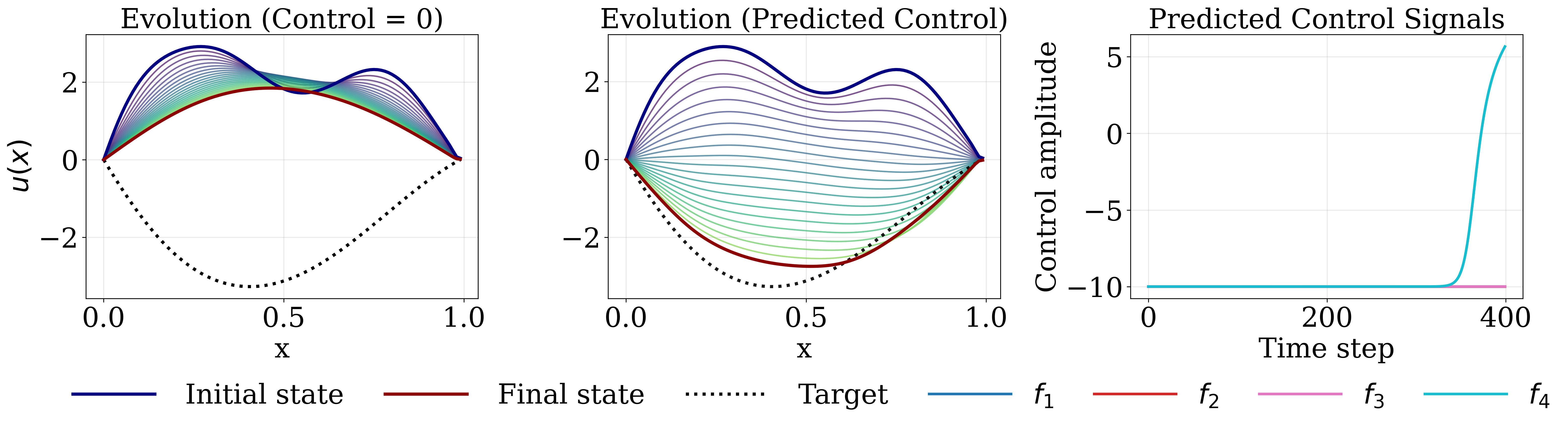
true solver The same policy driving the Crank-Nicolson solver.
learned dynamics Curvature suppressed relative to the uncontrolled shock-forming trajectory.
true solver The same policy driving the upwind Burgers solver.
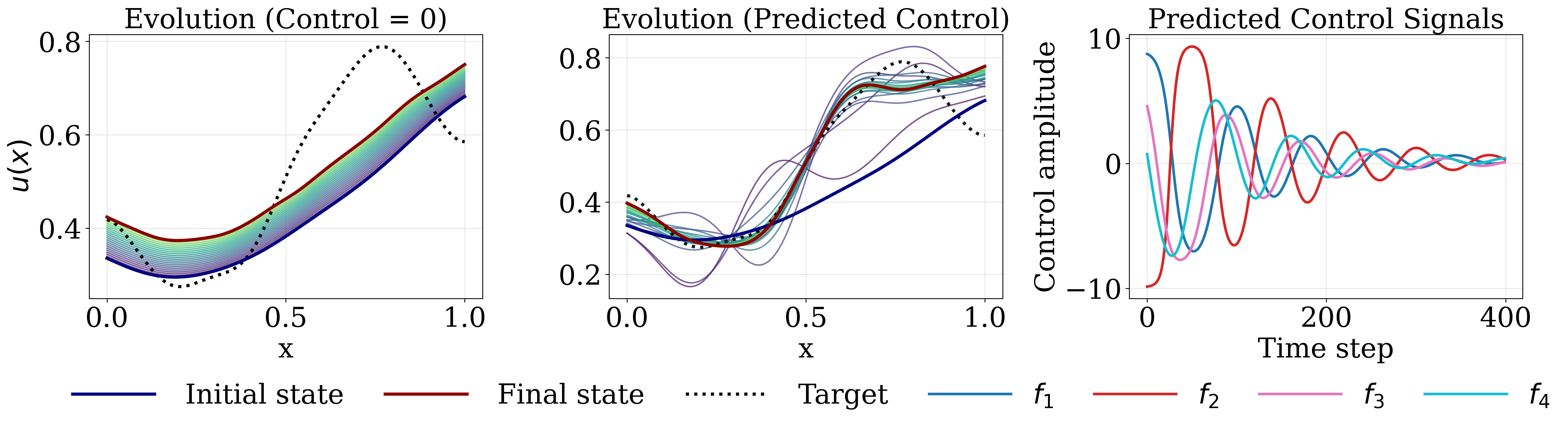
learned dynamics The policy counteracts the nonlinear reaction term driving the state toward $u\equiv 1$.
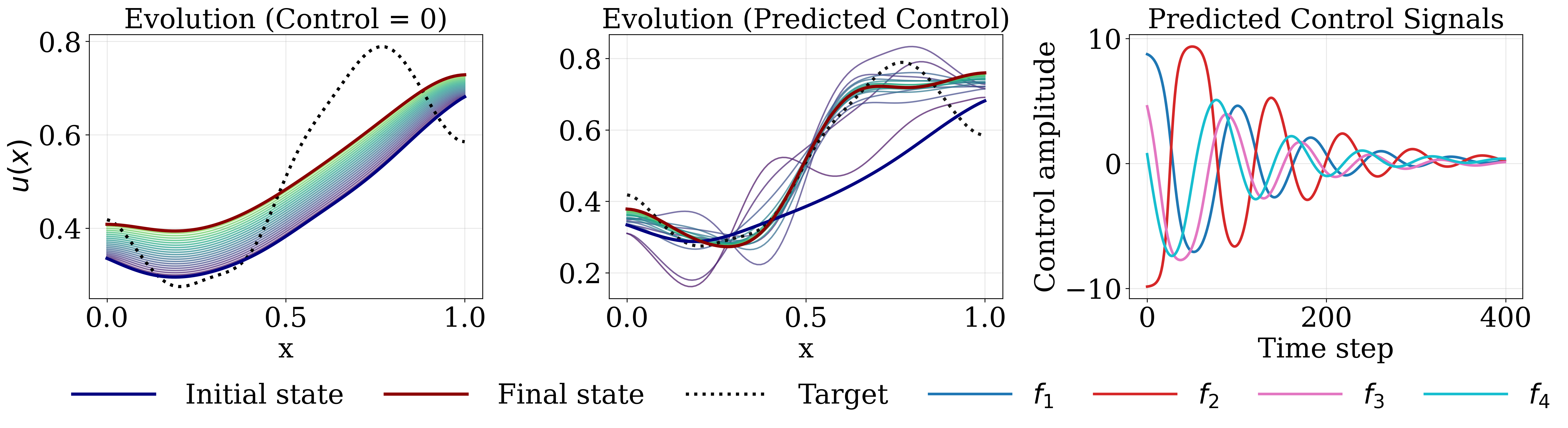
true solver The same policy driving the backward-Euler/Newton solver.
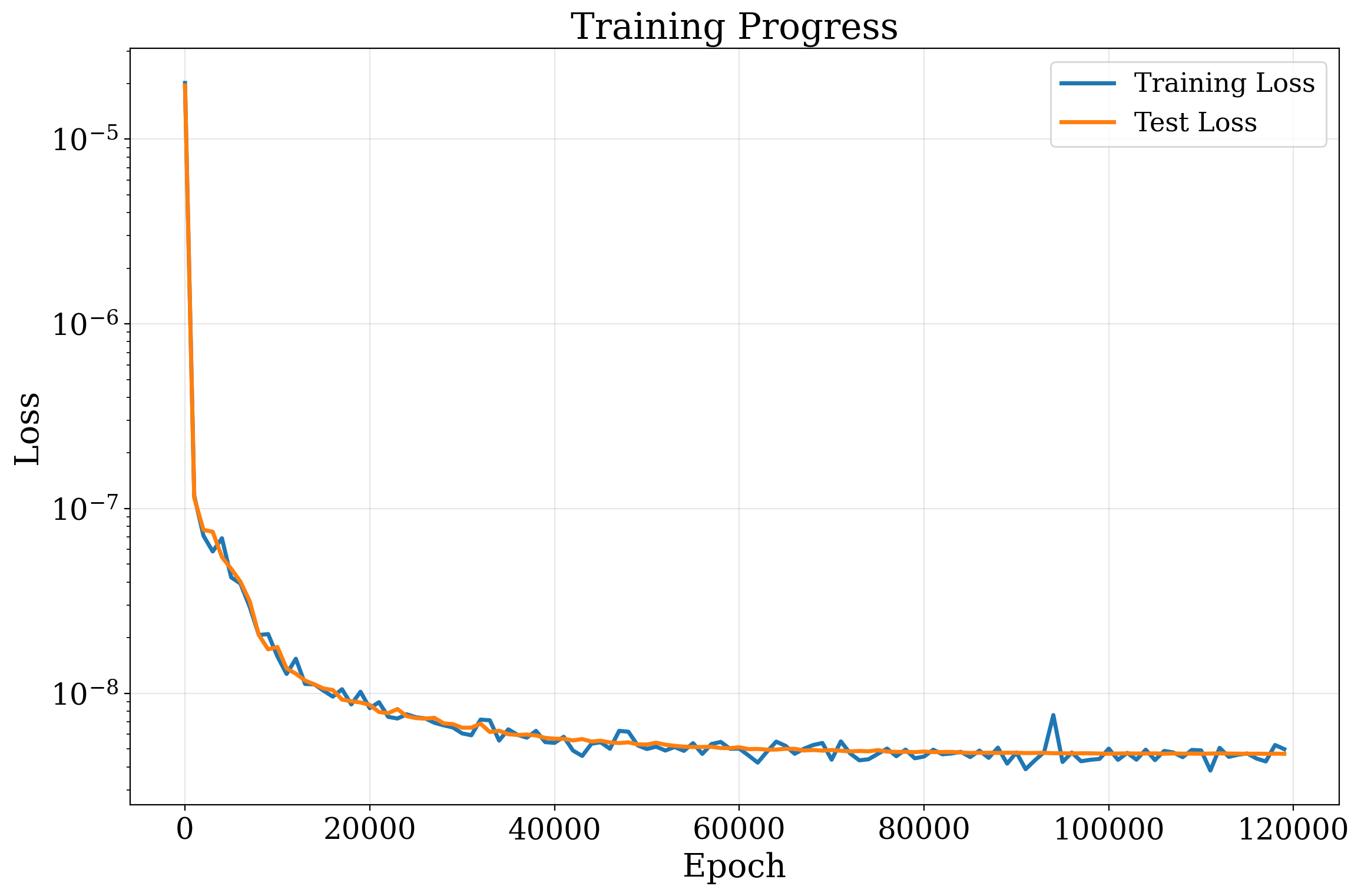
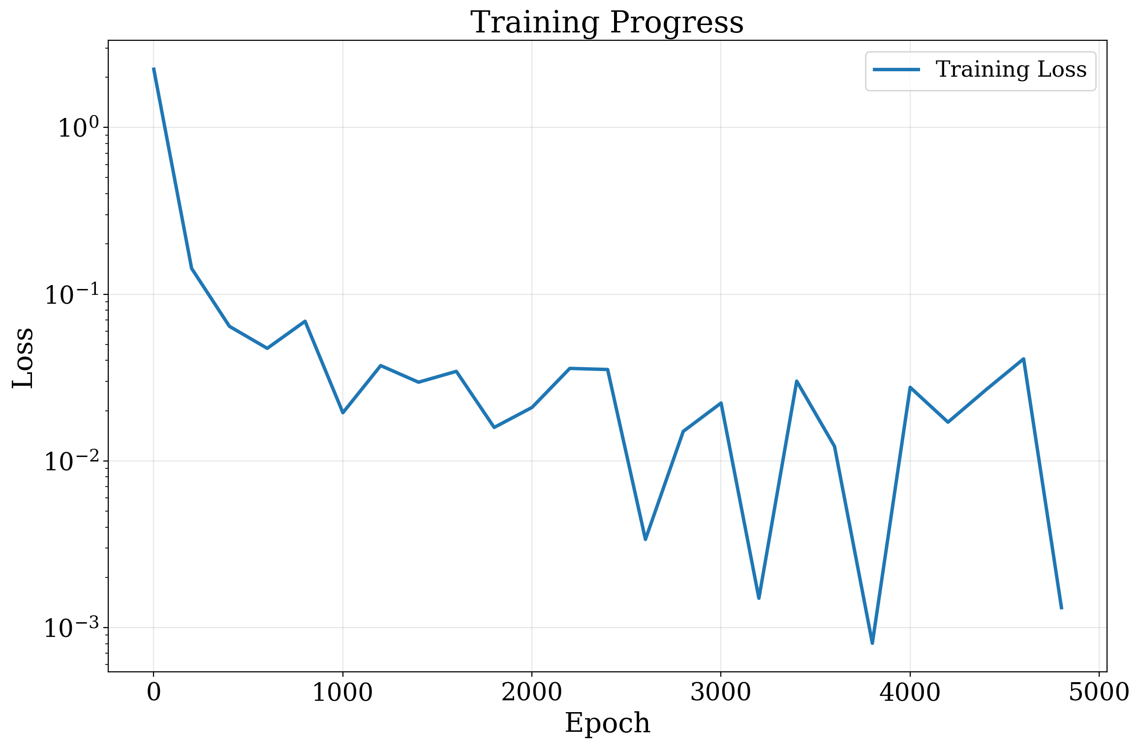
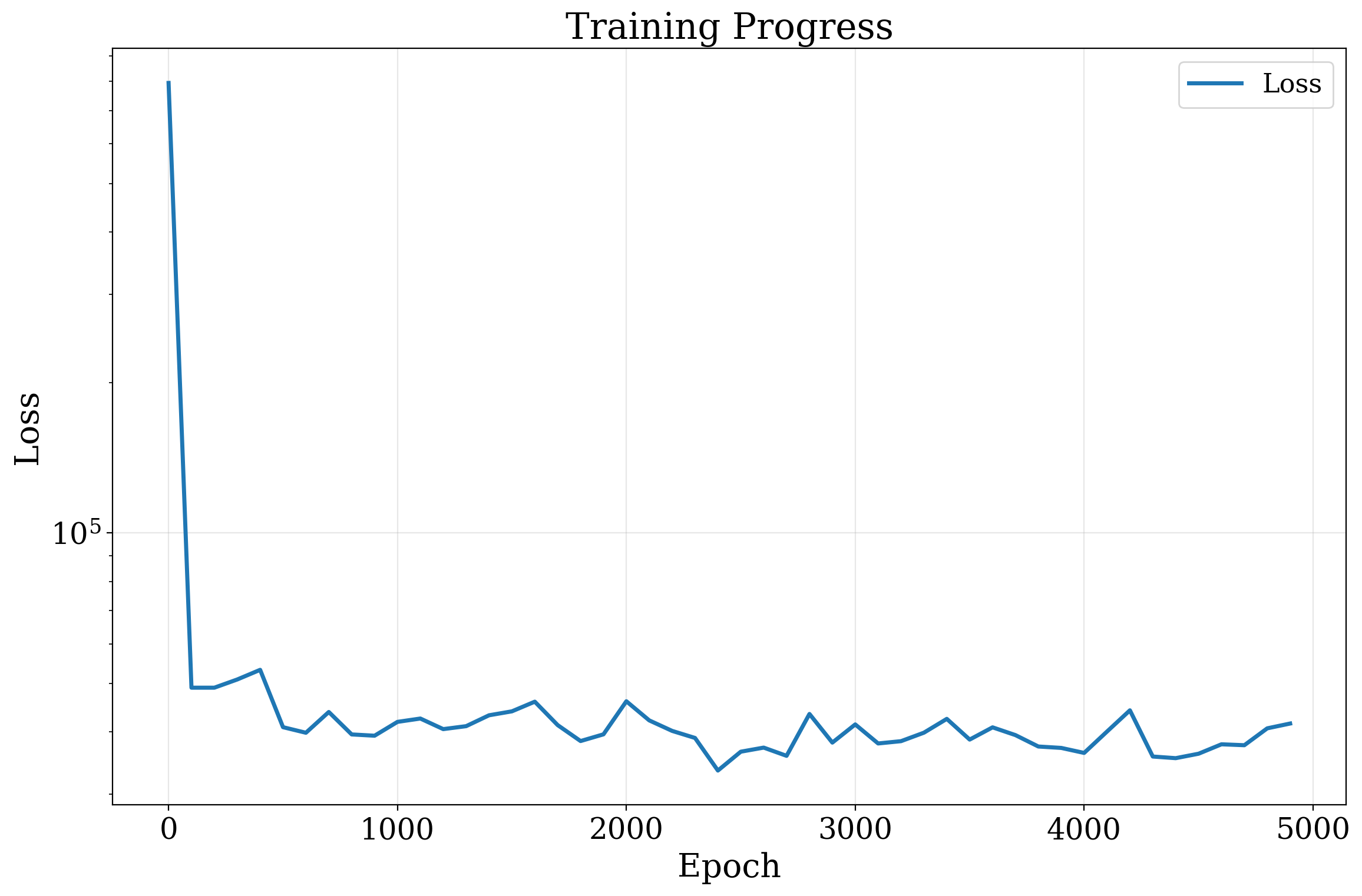
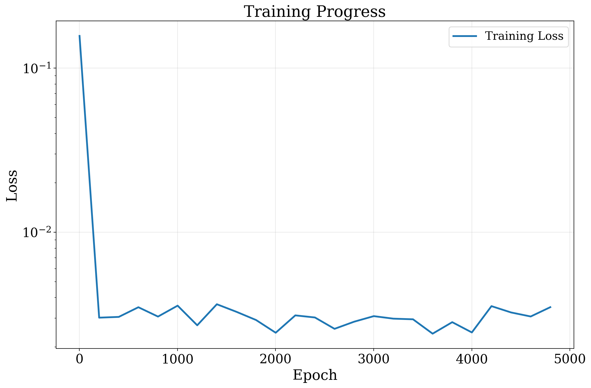
Stage 1 fits the surrogate to trajectory data. Stage 2 freezes it and fits the policy through differentiable rollouts. Note that the policy objective needs no labelled controls at all.
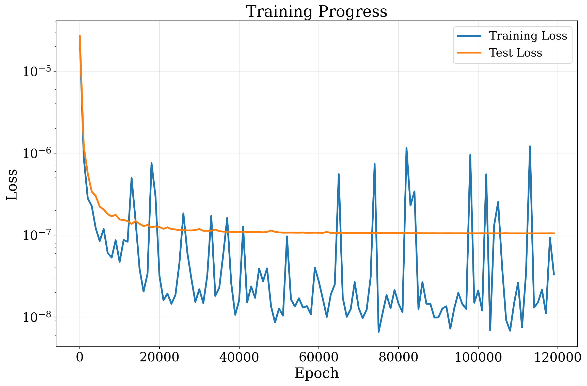
Heat
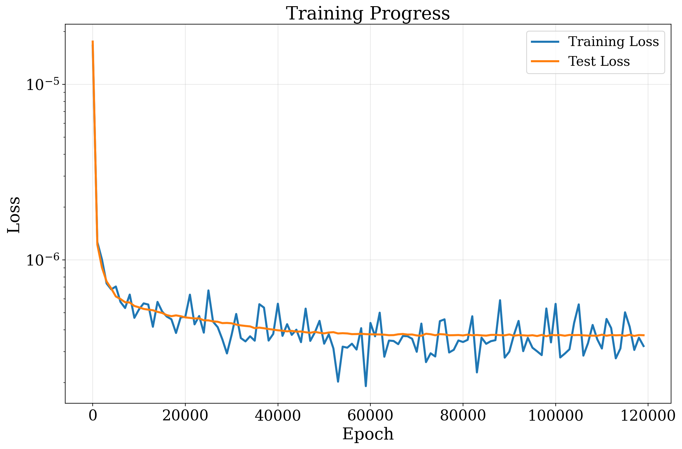
Burgers'
Reaction-diffusion
Heat: terminal tracking MSE
Burgers': accumulated curvature
Reaction-diffusion: terminal tracking MSE
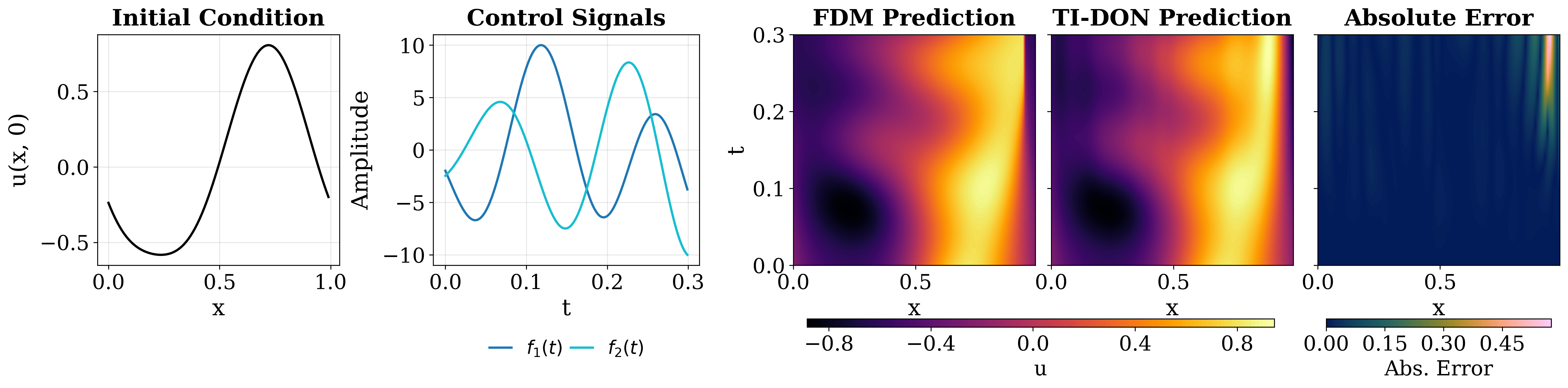
Relative $L_2$ error of the TI-DeepONet against the numerical solver over full trajectories.
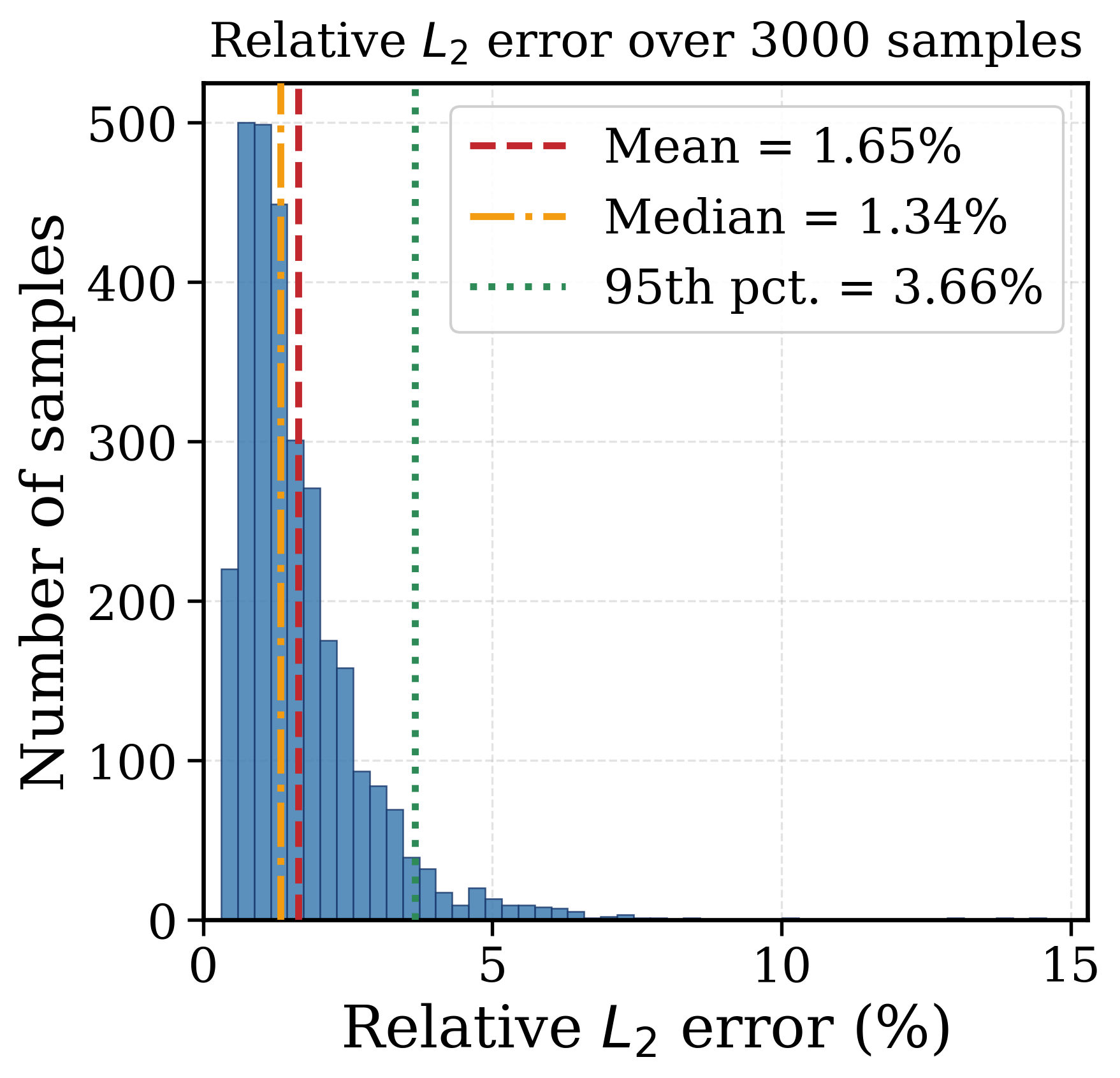
Heat
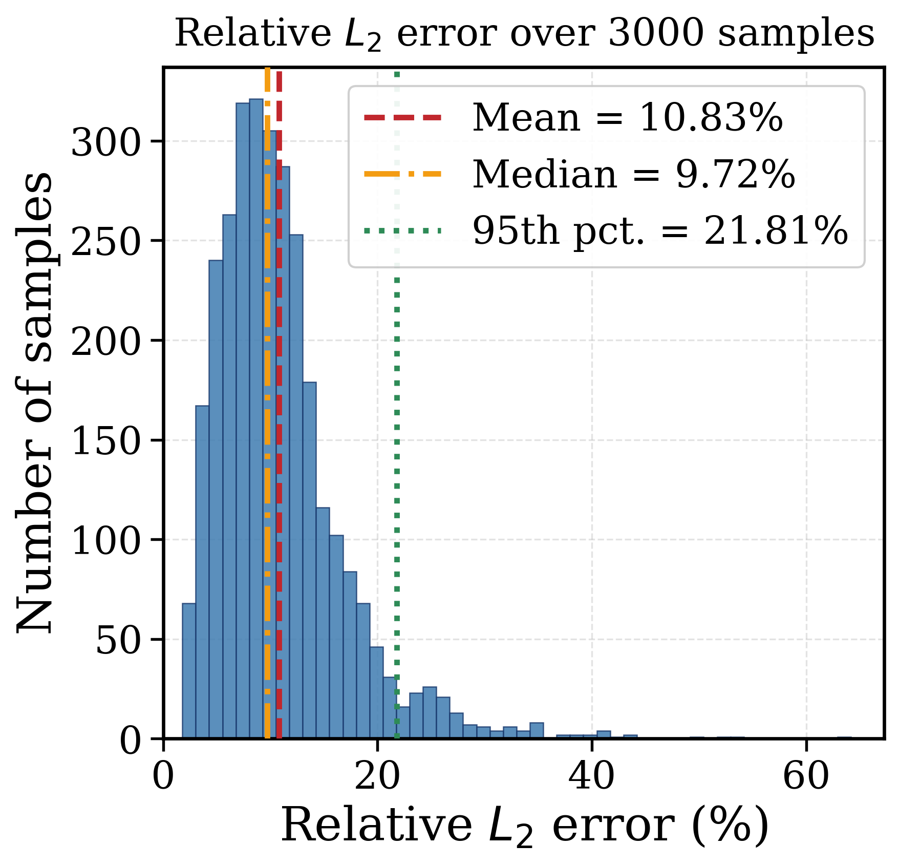
Burgers'
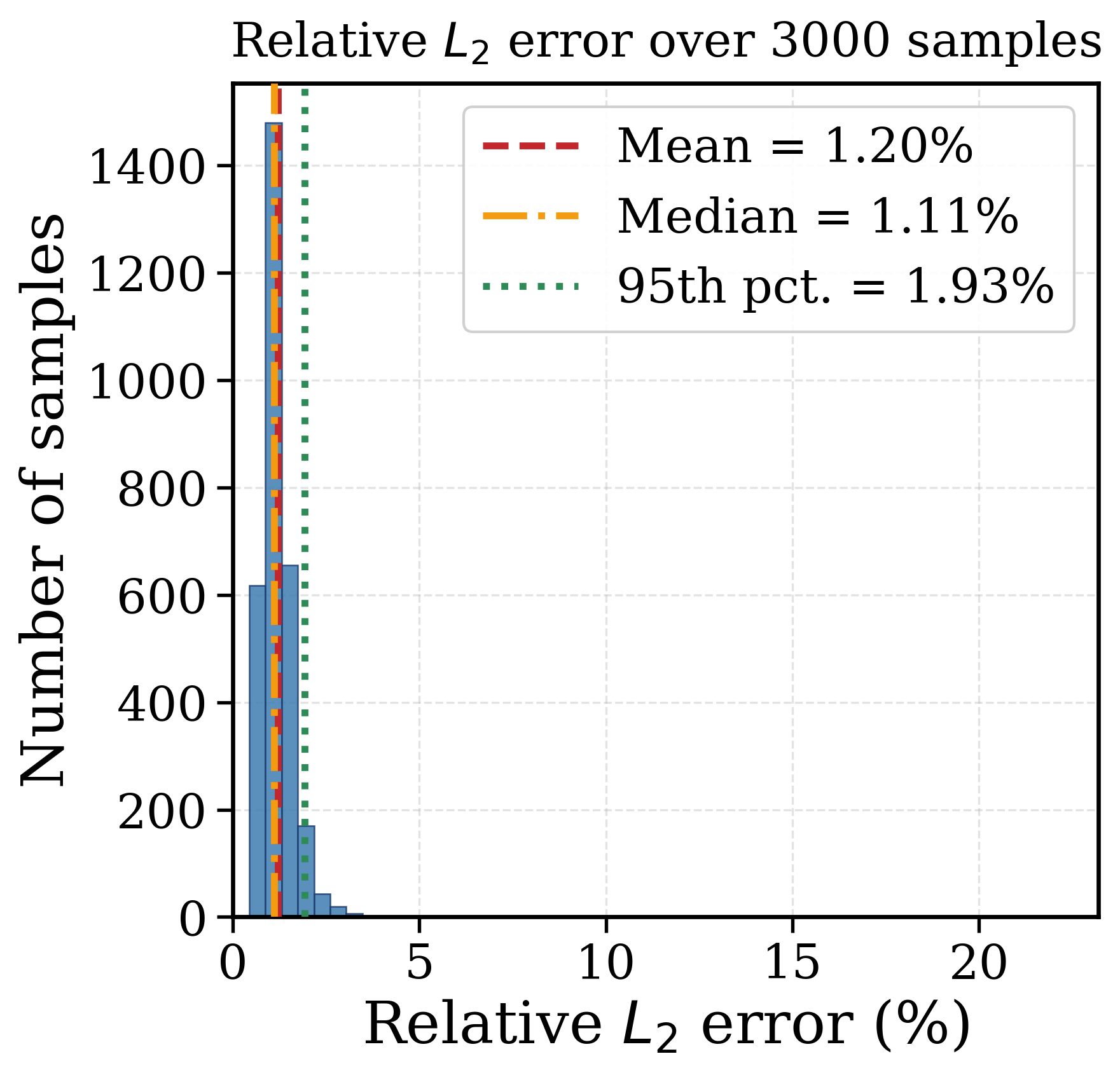
Reaction-diffusion
Pretrained checkpoints are in the repository, so the demo notebooks run on CPU in a few minutes with no dataset download. Open one in Google Colab and there is nothing to install — the first cell clones the repository into the Colab runtime for you.
| System | Run a pretrained policy | Train the policy yourself |
|---|---|---|
| Heat equation |
 |
|
| Burgers' equation |
|
|
| Reaction–diffusion |
|
|
01_control_demo.ipynbLoads the pretrained policy, generates fresh test cases, and validates on the true
numerical solver. Change one SEED for a new set of test cases.
02_train_dpc.ipynbTrains a policy from scratch through the frozen TI-DeepONet. Short schedule by default so it finishes quickly on CPU.
git clone https://github.com/Centrum-IntelliPhysics/PDEControl_DPC.git
cd PDEControl_DPC
pip install -r requirements.txt

cd HE_TT && jupyter notebook 01_control_demo.ipynb
The ~2.4 GB training datasets, needed only to retrain a surrogate from scratch,
are on
Hugging Face,
fetched with python download_data.py.
@misc{sarkar2025learningcontrolpdesdifferentiable,
      title={Learning to Control PDEs with Differentiable Predictive Control and Time-Integrated Neural Operators},
      author={Dibakar Roy Sarkar and J\'an Drgo\v{n}a and Somdatta Goswami},
      year={2025},
      eprint={2511.08992},
      archivePrefix={arXiv},
      primaryClass={cs.CE},
      url={https://arxiv.org/abs/2511.08992},
}